Applications of Derivatives

One of the most powerful uses of derivatives is analyzing the behavior of functions. By examining the derivative, we can determine where a function is increasing or decreasing, which provides insight into how outputs change as inputs vary. Derivatives provide an indication of when a function is increasing or decreasing by way of the slope of the tangent line. This is especially useful in fields such as economics, physics, biology and environmental applications, where understanding growth, decline, and rates of change is essential.

Another application of derivatives is finding maxima and minima, often referred to as optimization. These points represent the highest or lowest y-values a function can take within a certain interval. Identifying such values allows us to solve real-world problems, such as maximizing profit, minimizing cost, or determining the most efficient design of a system.

Derivatives also help us study the concavity of a function, which describes the curvature of a graph. Concavity provides information about the “shape” of a function’s behavior and helps distinguish between different types of turning points, such as local maxima or minima. Altogether, these applications of derivatives form a toolkit that allows us to describe, predict, and optimize the behavior of systems across many disciplines.

The video below provides more details and explanations for using the derivative to determine increasing, decreasing intervals, identify maxima and minima and determine concavity.

Derivatives represent one of the most widely used concepts in calculus. Derivative functions provide a basis for understanding how quantities change, which is essential for analyzing functions and solving real-world problems. The derivative of a function can be interpreted as its instantaneous rate of change, but beyond this definition, derivative allow us to

determine critical aspects of a function’s behavior. Among the most important applications are finding where a function is increasing or decreasing, locating maxima and minima, and determining concavity. Together, these tools give us the ability to analyze the shape and trends of a function, predict outcomes, and optimize processes.

In business applications, these concepts are widely used to maximize profit and minimize cost, in engineering to optimize designs, in environmental science to model population growth, and in physics to understand motion and forces. This section provides a detailed refresher on these applications of derivatives, complete with step-by-step examples, explanations, and connections to real-world scenarios.

1. Using Derivatives to Determine Increasing and Decreasing Functions

The derivative of a function provides insight into whether the function is increasing or decreasing at a given point. If the derivative is positive on an interval, the function is increasing on that interval. If the derivative is negative, the function is decreasing. This is known as the First Derivative Test. By finding the intervals of increase and decrease, we can sketch a more accurate picture of the function’s overall behavior.

Refer to the graph below for examples of increasing and decreasing intervals of a function:

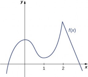
For this figure, the graph increases for the x-interval from -∞ to x = 0. The graph also increases the x-interval from x = 1 to x = 2.The graph decreases for the x-interval from x = 0 to x = 1 and also decreasing for the interval from x = 2 to ∞

Understanding these intervals is essential in real-world problems. For example, in economics, determining when revenue is rising or falling helps businesses adjust production. In physics, analyzing when velocity is positive or negative helps describe the direction of motion of an object.

Here are the step to finding increasing or decreasing intervals for a function using the first derivative test.

Determine the derivative function, f’(x)
Set this derivative function equal to zero, and solve for x. These x-values are called critical points (also called critical numbers). A critical point is an x-value where a derivative function is zero, or a derivative function is undefined. Thus a critical point c of a function is such that f’(c) = 0, or f’(c) is undefined.
Consider the x-intervals formed when using these critical points. Select an arbitrary x-value as a test point in each of these intervals.
Substitute this x-value into the derivative function. If the value of the derivative is positive, this indicates the interval represents an increasing interval. If the value of the derivative is negative, this indicates the interval represents a decreasing interval.

Example 1: Finding Intervals of Increase and Decrease

Consider the function f(x) = x³ – 6x² + 9x.

Step 1: Differentiate the function.
f′(x) = 3x² – 12x + 9

Step 2: Solve for critical points by setting f′(x) = 0.
3x² – 12x + 9 = 0
Divide by 3: x² – 4x + 3 = 0
So, (x – 1)(x – 3) = 0 → x = 1, 3

Step 3: Test intervals around the critical points.
For x < 1, choose x = 0: f′(0) = 9 > 0 (increasing).
For 1 < x < 3, choose x = 2: f′(2) = –3 < 0 (decreasing).
For x > 3, choose x = 4: f′(4) = 9 > 0 (increasing).
Thus, the function is increasing on (–∞, 1) and (3, ∞), and decreasing on (1, 3).

Example 2: Revenue Growth

Suppose a company’s revenue function is given by R(x) = –2x² + 20x, where x is the number of products sold (in hundreds). To determine when revenue is increasing or decreasing:

Step 1: Differentiate.
R′(x) = –4x + 20

Step 2: Solve for zero.
–4x + 20 = 0 → x = 5

Step 3: Test intervals.
For x < 5, choose a test value of 3, then R′(3) = 8, which is a value > 0 (increasing). For x > 5, choose a test value of 6, then R′(6) = -4, which is a value < 0 (decreasing).

Interpretation: Revenue increases until 500 units are sold, after which it begins to decline due to overproduction or market saturation.

2. Using Derivatives to Find Maxima and Minima

Maxima and minima, collectively called extrema, represent points where a function reaches its highest or lowest y-values. These extrema are important for optimization problems, such as maximizing profit, minimizing cost, or finding the optimal dimensions of a shipping container to minimize the amount of material used. The process typically involves finding critical points (where the derivative equals zero or is undefined) and then applying either the First or Second Derivative Test.

Example 3: Finding Local Maxima and Minima

Using the same function as the previous example, locate any maxima or minima: f(x) = x³ – 6x² + 9x:

Step 1: Critical points occur at x = 1 and x = 3. Step 2: Apply the First Derivative Test.

At x = 1, f′(x) changes from positive to negative → local maximum.
At x = 3, f′(x) changes from negative to positive → local minimum.

Step 3: Evaluate function values.
f(1) = 4 → local maximum at (1, 4).
f(3) = 0 → local minimum at (3, 0).

Example 4: Minimizing Cost

A manufacturer determines that the cost of producing x items is given by C(x) = 0.5x² – 20x

+ 400. Find the production level that minimizes cost. Step 1: Differentiate.

C′(x) = x – 20

Step 2: Solve for critical points. x – 20 = 0 → x = 20

Step 3: Second Derivative Test.
C″(x) = 1 > 0 → local minimum.

Thus, producing 20 items minimizes cost.

3. Concavity and Points of Inflection

The second derivative tells us about the concavity of a function. If f″(x) > 0, the graph is concave up (shaped like a cup). If f″(x) < 0, it is concave down (shaped like a cap). A point where the concavity changes is called an inflection point. Understanding concavity allows us to refine sketches of graphs and to interpret changes in acceleration, growth rates, or curvature in real-world phenomena.

Here are the step to finding concave up or concave down intervals for a function using the second derivative test.

Determine the first derivative function, f’(x). Then take the derivative again todetermine the second derivative function f’’(x)
Set this second derivative function equal to zero, and solve for x.
Consider the x-intervals formed when using x-values. Select an arbitrary x-value as a test point in each of these intervals.
Substitute this x-value into the second derivative function. If the value of the second derivative is positive, this indicates the interval represents a concave up interval. If the value of the second derivative is negative, this indicates the interval represents a concave down interval.

Example 5: Determining Concavity

For f(x) = x³ – 6x² + 9x:
Step 1: Find second derivative.
f″(x) = 6x – 12
Step 2: Solve f″(x) = 0.
6x – 12 = 0 → x = 2
Step 3: Test intervals.
For x < 2, f″(x) < 0 → concave down. For x > 2, f″(x) > 0 → concave up.
Thus, there is an inflection point at (2, f(2) = 2).

Example 6: Motion Analysis

Consider the position of a particle given by s(t) = t³ – 6t² + 9t.
Velocity: v(t) = s′(t) = 3t² – 12t + 9
Acceleration: a(t) = v′(t) = 6t – 12
By analyzing where v(t) is positive or negative, we know when the particle is moving forward or backward. By checking concavity with a(t), we determine whether the motion is speeding up or slowing down.

4. Extended Applications in Business, Science, and Engineering

Business Applications

In business, derivatives are indispensable tools. Companies often model revenue, cost, and profit functions to find the number of units that maximizes profit or minimizes cost. For example, if revenue grows quickly at first but slows later, the derivative helps pinpoint the production level where revenue peaks. Similarly, cost minimization problems often involve finding where the derivative of a cost function equals zero.

Example 7: Maximizing Profit

Suppose profit is modeled by P(x) = –2x² + 40x – 150, where x is in hundreds of units.

Step 1: Differentiate.
P′(x) = –4x + 40

Step 2: Solve for zero. x = 10

Step 3: Second derivative.
P″(x) = –4 < 0 → maximum.

Thus, maximum profit occurs at 1000 units. This type of analysis allows businesses to determine the optimal production level.

Environmental Applications

In environmental science, derivatives are used to analyze population dynamics, pollution levels, and rates of resource consumption. Logistic growth models, for example, use derivatives to determine when growth rates are fastest and when populations stabilize.

Example 8: Population Growth

Suppose population is modeled as P(t) = 1000 / (1 + e^–0.5t).
Step 1: Differentiate.
P′(t) = (500e^–0.5t) / (1 + e^–0.5t)^2

Step 2: Analyze growth.
The growth rate is maximized when the denominator is smallest, which occurs at t = 0.

Interpretation: At early stages, population growth accelerates. Eventually, the rate slows as resources become limited.

Engineering Applications

In engineering, derivatives help design systems that minimize material use while maximizing strength. For example, finding the optimal dimensions of a beam or minimizing drag on a vehicle often involves setting derivatives equal to zero and solving for optimal conditions.

Conclusion

Derivatives provide essential tools for understanding the shape and behavior of functions. By determining intervals of increase and decrease, we analyze trends. By finding maxima and minima, we optimize. By examining concavity and inflection points, we understand how functions bend and shift. Across business, science, engineering, and economics, these tools are indispensable for problem-solving. Mastering these applications equips students with the analytical skills to tackle challenges in both academic and real-world contexts.