Integration

Together with differentiation, the topic of integration is one of the central concepts in calculus and serves as a powerful tool for understanding and solving problems across mathematics, science, and engineering.
Integration can be thought of as the reverse process of differentiation: while derivatives measure rates of change, integrals allow us to accumulate or combine small quantities to find totals. This makes integration especially useful for determining areas, volumes, and other quantities that arise from continuous change. For example, integration can be used to calculate the area under a curve, the total distance traveled from a velocity function, or the work done by a force over a distance.
In environmental science applications, researchers might be interested to calculate volume of groundwater available in an aquifer, the spread of contaminants through soil, or the carbon stored in a forest ecosystem. In each case, integration allows environmental scientists to combine many small, variable changes into a meaningful total that can guide research and policy decisions.
Beyond these applications, integration is also essential in modeling real-world phenomena. In physics, it helps describe motion, energy, and fluid flow; in economics, it can be used to find consumer and producer surplus; in biology, it assists in modeling population growth and resource consumption. Conceptually, integration is about summing infinitely many tiny contributions to obtain a meaningful whole. There are various methods for integration that help to integrate more complex functions such as substitution, integration by parts, and numerical approximation methods.
The video below provides more details and explanations for the topic of integration together with several worked-out examples.
Along with differentiation, the topic of integration is a fundamental concept in calculus. While differentiation explores rates of change and instantaneous behaviors of functions, integration provide information regarding the accumulation or summation of quantities. Most commonly, integration is used to determine the area under a curve, but its utility extends beyond this geometric interpretation. Integration is used across mathematics, physics, business, engineering, and environmental science to solve problems involving areas, volumes, totals, averages, and more. This section provides a review of integration, starting with its formal definition, geometric meaning, and notation. The power rule for integration is also discussed, and multiple worked-out examples are provided. Applications to business and environmental science are also included.
The Concept of Integration
Integration can be thought of as a process that is the inverse or opposite of the differentiation process.
To emphasize this, integration is also sometimes referred to as the “antiderivative”.
One way to think about integration is to consider a derivative function \( f'(x) \).
If you know \( f'(x) \), integration is the process to work backwards to find \( f(x) \)
Example: You are given that the derivative function \( f'(x) = 2x \). The process of integration asks: what is \( f(x) \)
Notice that if you are given that \( f'(x) = 2x \), the original function \( f(x) = x^2 \), since the derivative of \( x^2 \) is \( 2x \).
However all of these could be valid answers for \( f(x) \):
\( f(x) = x^2 \)
\( f(x) = x^2 + 9 \)
\( f(x) = x^2 – 15 \)
\( f(x) = x^2 + C \)
Note: Once an antiderivative of a function \( f \) is known, then other antiderivatives of \( f \) can be written by adding an arbitrary constant \( C \)
The process of finding all antiderivatives of a function is generally referred to as the process of integration.
We use the symbol \( \int \) ,called an integral sign
\[ \int f(x)\,dx = F(x) + C \]
So we could write: \( \int 2x\,dx = x^2 + C \)
In this notation \( f(x) \) is the derivative function and \( F(x) \) is the antiderivative function
The integral of a function gives the accumulated total of its values over an interval, often corresponding to the area under the curve of the function on a graph. Consider a continuous real-valued function \( f(x) \); the integral of \( f(x) \) from \( a \) to \( b \), denoted
\[ \int_a^b f(x)\,dx \]
represents the signed area between the curve \( y=f(x) \), the x-axis, and the vertical lines \( x = a \) and \( x = b \).
Integrals as Area Under a Curve
Graphically, imagine breaking the area under the curve into thin rectangles, each of infinitesimal width (dx). The height of each rectangle is determined by the function \( f(x) \), and its width is dx. The sum of the areas of these rectangles is approximated (for a large number of rectangles), and integration formalizes this sum as the exact area:
\[ \text{Area} \approx \sum f(x_i)\,\Delta x \]
as \( \Delta x \to 0 \)
so
\[ \text{Area} = \int_a^b f(x)\,dx \]
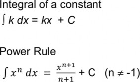
Integration Rules
Two important rules for integration are summarized below:
Types of Integrals
Indefinite Integrals
An indefinite integral is denoted
\[ \int f(x)\,dx \]
and gives the general antiderivative of \( f(x) \). The result includes an arbitrary constant, \( C \):
\[ \int f(x)\,dx = F(x) + C \]
because differentiating a constant yields zero, and all possible antiderivatives differ by a constant. For example,
\[ \int x^2\,dx = \frac{x^3}{3} + C \]
Definite Integrals
A definite integral has specified limits (aa and bb):
\[ \int_a^b f(x)\,dx \]
and computes the (possibly signed) area under the curve from \( x=a \) to \( x=b \). The result is a number, not a function:
\[ \int_a^b f(x)\,dx = F(b) – F(a) \]
where \( F(x) \) is any antiderivative of \( f(x) \).
Example 1: Area under a Graph
Let \( f(x) = 2x+1 \)
Find the area under this curve for x between 1 and 2. The area under this curve is
\[ \int_1^2 (2x + 1)\,dx \]
Compute the antiderivative:
- The integral of 2x is \( x^2 \)
- The integral of 1 is \( x \).
So,
\[ \int (2x+1)\,dx = x^2 + x + C \]
To evaluate the lower and upper bounds, first plug in the upper bound into this function “ x2 + x “ Then plug in the lower bound, Then subtract the two results , as follows:
Applying the limits:
\[ (2^2 + 2) – (1^2 + 1) \]
= 6 – 2
= 4
The conclusion is that the area under \( f(x) \) from \( x=1 \) to \( x=2 \) is 4 square units.
Example 2: Power Rule
Find \( \int x^3\,dx \)
Solution:
- n=3
- By the power rule,
- \[ \int x^3\,dx = \frac{x^4}{4} + C \]
Example 3: Negative Exponent
Find \( \int x^{-2}\,dx \)
Solution:
- n=-2
- By the rule,
- \[ \int x^{-2}\,dx = \frac{x^{-1}}{-1} + C = -\frac{1}{x} + C \]
Example 4: Fractional Exponent
Find \( \int \sqrt{x}\,dx \)
Solution:
- Rewrite \( \sqrt{x} \) as \( x^{1/2} \)
- n=1/2
- By the rule,
- \[ \int x^{1/2}\,dx = \frac{2}{3}x^{3/2} + C \]
More Worked Examples
Example 1: Polynomial Integration
Integrate \( \int (2x^2 – 3x + 4)\,dx \)
Solution:
\[ \int (2x^2 – 3x + 4)\,dx = \frac{2x^3}{3} – \frac{3x^2}{2} + 4x + C \]
Example 2: Definite Integral for Area
Find the area under \( f(x)=x^2 \) between \( x=1 \) and \( x=2 \):
Solution:
\[ \int_1^2 x^2\,dx = \left[\frac{x^3}{3}\right]_1^2 = \frac{7}{3} \]
Applications
Business
- Revenue, Cost, and Profit: Integration enables business analysts to compute total revenue from a marginal revenue function or total cost from a marginal cost function over a quantity interval.
Accumulation: For example, total sales over time when given a sales rate function.
Continuous Compounding: Integrals are used in finance models for continuously compounded interest, market equilibrium, and more.
Environmental Science
- Total Emissions: Calculate cumulative pollutant discharge from a rate function.
- Resource Management: Integrals help determine total resource usage or replenishment over time, such as water, energy, or soil nutrients.
Modeling Population Growth: The accumulation of population changes can be described with integral calculus.
Area and Volume Calculations: For modeling land area, watershed volumes, or area under concentration-time curves in environmental monitoring.
