Extrema and Optimization

A function of several variables is a function that takes multiple inputs and produces a single output, often written as f(x, y) or f(x, y, z) . These functions describe surfaces in three or higher dimensions. Understanding these functions is fundamental for studying real-world phenomena, such as temperature distribution, fluid flow, environmental monitoring and economic models.
In multivariable calculus, the study of extrema and optimization for three-dimensional functions focuses on finding points where a function reaches its highest or lowest values within a given region. These functions typically depend on two independent variables, such as , and describe surfaces in three-dimensional space. Understanding where these surfaces reach maximum or minimum values is essential for solving real-world problems in science, engineering, economics, and environmental modeling.
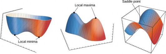
The process begins by identifying critical points, where the rates of change in all directions are zero. These points may represent local maxima, local minima, or saddle points—locations where the surface curves upward in one direction and downward in another. Determining the nature of each critical point involves analyzing how the function behaves nearby, often through second-derivative tests or related methods.
Optimization extends these ideas to applied settings, where the goal is to maximize or minimize a quantity subject to constraints. For instance, one might maximize profit, minimize material usage, or optimize environmental outcomes within physical or financial limits.
The video below reviews methods to determine these extrema and includes several worked out examples.
In multivariable calculus, the study of extrema and optimization for three-dimensional
functions focuses on finding points where a function reaches its highest or lowest values within a given region. These functions typically depend on two independent variables, such as 𝑓(𝑥, 𝑦), and describe surfaces in three-dimensional space.
These concepts generalize single-variable calculus ideas such as local maxima, minima, and optimization to higher dimensions. This analysis in three dimensions is critical for modeling real-world applications. In business, engineering, and environmental science, optimization problems involving functions of several variables are common—for example, minimizing production costs, maximizing efficiency, or modeling environmental impacts.
The process begins by identifying critical points, where the rates of change in all directions are zero. These points may represent local maxima, local minima, or saddle points. Saddle points are locations where the surface curves upward in one direction and downward in
another (similar to the shape of a saddle). Determining the nature of each critical point involves analyzing how the function behaves nearby, often through second-derivative tests or related methods.
Once these critical points are identified using first partial derivatives, then second derivatives are used to help classify whether the critical point is a local minimum, local maximum, or saddle point.
Understanding where these surfaces reach maximum or minimum values is essential for solving real-world problems in science, engineering, economics, and environmental modeling.
Functions of Two Variables
A function of two variables is denoted as z = f(x, y), where each point (x, y, z) represents a value on a surface in three-dimensional space. The graph of z = f(x, y) is a surface that can have peaks (maxima), valleys (minima), and saddle points (points that are maxima in one direction and minima in another).
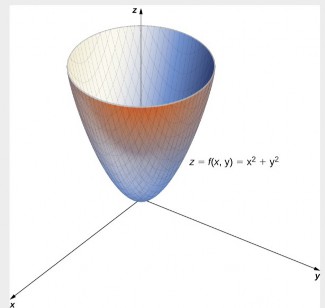
Example of function of two variables:
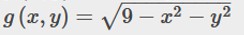
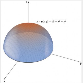
Another example of function of two variables:
Partial Derivatives
To study how a surface changes in different directions, we compute partial derivatives. The partial derivative of f with respect to x, denoted as fₓ(x, y), measures the rate of change of f in the x-direction while keeping y constant. Similarly, fᵧ(x, y) measures the rate of change in the y-direction.
Partial derivatives are expressed using the following notation:
fₓ(x, y) = ∂f/∂x and fᵧ(x, y) = ∂f/∂y
The idea to keep in mind when calculating partial derivatives is to treat all independent variables, other than the variable with respect to which we are differentiating, as constants. Then proceed to differentiate as with a function of a single variable.
For example, to calculate ∂f/∂x take the derivative of x, but treat the variable y as a constant.
Critical Points
One of the most useful applications for derivatives of a function of one variable is the determination of maximum and/or minimum values.
For functions of a single variable, we define critical points as the values of the function when the derivative equals zero or does not exist. For functions of two or more variables, the concept is essentially the same, except for the fact that we are now working with partial derivatives.
Critical points occur where both partial derivatives are zero or undefined, i.e.: fₓ(x, y) = 0 and fᵧ(x, y) = 0
At these points, the surface may have a local maximum, local minimum, or a saddle point as shown in the figure below.
To classify them, we use the Second Partial Derivative Test.
The Second Partial Derivative Test
Let f(x, y) have continuous second partial derivatives near a critical point (a, b). Define the value D, as follows:
D = fₓₓ(a, b) * fᵧᵧ(a, b) − [fₓᵧ(a, b)]²
Where:
fxx is the second partial derivative with respect to 𝑥.
fyy is the second partial derivative with respect to 𝑦.
fxy is the second partial derivative with respect to 𝑦 𝑜𝑓 𝑓𝑥.
Once the value of D is calculated and the value of fₓₓ is calculated, then the nature of the critical point is determined as follows:
- If D > 0 and fₓₓ(a, b) > 0, then f has a local minimum at (a, b).
- If D > 0 and fₓₓ(a, b) < 0, then f has a local maximum at (a, b).
- If D < 0, then (a, b) is a saddle point.
- If D = 0, the test is inconclusive.
Example : Finding and Classifying Critical Points
Find and classify the critical points of f(x, y) = x² + y² − 4x − 6y + 13.
Step 1: Compute partial derivatives:
fₓ = 2x − 4, fᵧ = 2y − 6
Step 2: Set partial derivatives equal to zero:
2x − 4 = 0 → x = 2
2y − 6 = 0 → y = 3
So the critical point is (2, 3).
Step 3: Compute second partial derivatives:
fₓₓ = 2, fᵧᵧ = 2, fₓᵧ = 0
Step 4: Compute the value of D:
D = (2)(2) − (0)² = 4 > 0
Since D > 0 and fₓₓ = 2 > 0, the point (2, 3) is a local minimum.
Example : Saddle Point
Find and classify the critical points of f(x, y) = x² − y².
Step 1: Compute partial derivatives:
fₓ = 2x, fᵧ = −2y
Step 2: Set partial derivatives equal to zero:
2x = 0 → x = 0
−2y = 0 → y = 0
So the critical point is (0, 0).
Step 3: Compute second partial derivatives:
fₓₓ = 2, fᵧᵧ = −2, fₓᵧ = 0
Step 4: Compute the discriminant:
D = (2)(−2) − 0² = −4 < 0
Since D < 0, the point (0, 0) is a saddle point. Graphically, the surface looks like a saddle—it curves upward in one direction and downward in the other.
Environmental Science Application
Optimization techniques are frequently used in environmental modeling. For instance, minimizing pollution concentration or maximizing biodiversity subject to resource constraints can be modeled using functions of several variables.
Example: Suppose the pollution concentration in a region is modeled by:
P(x, y) = x² + y² − 8x − 6y + 25,
where (x, y) represents the coordinates of a monitoring station. To find the location that minimizes pollution, we follow the same procedure as before.
Compute partial derivatives:
Pₓ = 2x − 8, Pᵧ = 2y − 6
Set both equal to zero:
2x − 8 = 0 → x = 4, 2y − 6 = 0 → y = 3
Compute second derivatives:
Pₓₓ = 2, Pᵧᵧ = 2, Pₓᵧ = 0 → D = 4 > 0, Pₓₓ > 0
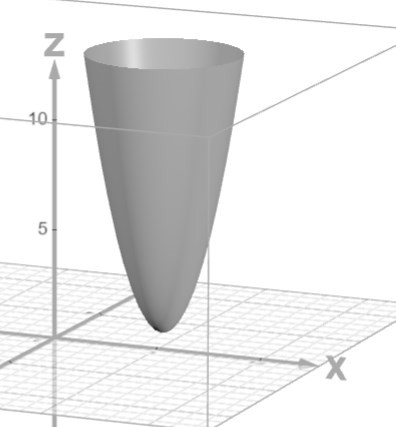
Therefore, the minimum pollution concentration occurs at (4, 3). Substituting into the function gives P(4, 3) = 16 + 9 − 32 − 18 + 25 = 0. Hence, pollution is minimized at this point.
A graph of this function is shown below, confirming that the graph exhibits a minimum.
Summary
Extrema and optimization in three-dimensional calculus extend the one-variable methods to three dimensional surfaces. Through the use of partial derivatives, and the second derivative test, we can identify maxima, minima, and saddle points both in theoretical and applied contexts. These tools are widely applied in scientific, economic, environmental and engineering fields. For instance, economists use optimization to maximize profit or minimize cost functions, while environmental scientists use similar methods to find equilibrium points in models of pollution dispersion or habitat sustainability.
