Line Integrals and Surface Integrals

In three-dimensional calculus, line integrals and surface integrals extend the concept of integration beyond simple regions in the plane to curves and surfaces in space. These tools allow us to measure quantities such as work done by a force field along a path, or the flow of a vector field across a surface—ideas that are fundamental in physics, engineering, and applied mathematics. Vector fields are used to describe many physical concepts, such as gravitation and electromagnetism, where these fields affect the behavior of objects over a large region of a plane or of space. Vector fields are also useful for dealing with large-scale behavior such as atmospheric storms or deep-sea ocean currents.
A line integral evaluates a function or vector field along a curve in space. Instead of summing values over an interval on the x-axis, a line integral sums contributions along a path that may curve or twist in three dimensions. This process captures how a quantity—like force, mass, or heat—accumulates along that path. For example, the work done in moving an object along a trajectory within a force field can be expressed using a line integral.
A surface integral generalizes the idea of a double integral to curved surfaces in space. It measures how a scalar or vector field interacts with a surface—such as calculating the total electric flux passing through a surface or the rate at which fluid flows across it.
Together, line and surface integrals form the foundation for theorems in vector calculus, including Green’s, Stokes’, and the Divergence Theorem, which provide connections between integrals over curves, surfaces, and regions in space.
The video below reviews methods to determine line integrals and surface integrals and includes several worked out examples.
Line integrals extend the concept of integration beyond simple regions in the plane to curves and surfaces in space. These tools allow us to measure quantities such as work done by a force field along a path, or the flow of a vector field across a surface. A line integral evaluates a function or vector field along a curve in space. Instead of summing values over an interval on the x-axis, a line integral sums contributions along a path that may curve or twist in three dimensions.
A surface integral generalizes the idea of a double integral to curved surfaces in space. It measures how a scalar or vector field interacts with a surface—such as calculating the total electric flux passing through a surface or the rate at which fluid flows across it.
Line Integrals
A line integral is used to integrate a function along a curve in three-dimensional space. Suppose we have a curve C parameterized by f(r(t) = x(t) i + y(t) j + z(t) k for (a ≤ t ≤ b).
The line integral of a scalar function \( (f(x,y,z)) \) along this curve is defined as:
\[ \int_C f(x,y,z),ds \]
Here, \( ds \) represents the differential arc length along the curve, given by:
\[ ds = \sqrt{\left(\frac{dx}{dt}\right)^2 + \left(\frac{dy}{dt}\right)^2 + \left(\frac{dz}{dt}\right)^2},dt. \]
Consequently, the line integral can be expressed in terms of the parameter (t) as:
\[ \int_a^b f(x(t),y(t),z(t))\sqrt{\left(\frac{dx}{dt}\right)^2 + \left(\frac{dy}{dt}\right)^2 + \left(\frac{dz}{dt}\right)^2} dt. \]
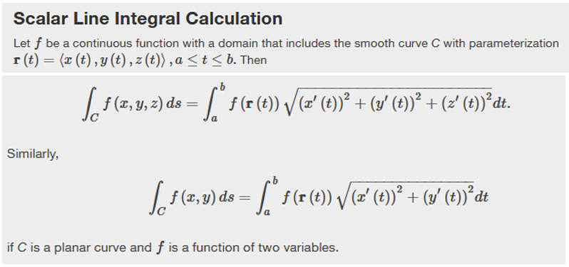
Scalar Line Integral
Note that a line integral does not depend on the parameterization r(t) of C. As long as the curve is traversed exactly once by the parameterization, the area of the sheet formed by the function and the curve is the same. This same kind of geometric argument can be extended to show that the line integral of a three-variable function over a curve in space does not depend on the parameterization of the curve.
Note that in a scalar line integral, the integration is done with respect to arc length s, which can make a scalar line integral difficult to calculate. To make the calculations easier, we can translate ∫C f ds to an integral with a variable of integration that is t.
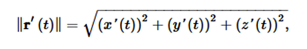
Let r(t)=⟨x(t), y(t), z(t)⟩ for a ≤ t ≤ b be a parameterization of C. Since we are assuming that C is smooth, r′(t)=⟨x′(t), y′(t), z′(t)⟩ is continuous for all t in [a, b]. In particular, x'(t),y'(t), and z'(t) exist for all t in [a, b].
This leads to the following theorem for evaluating a scalar line integral:
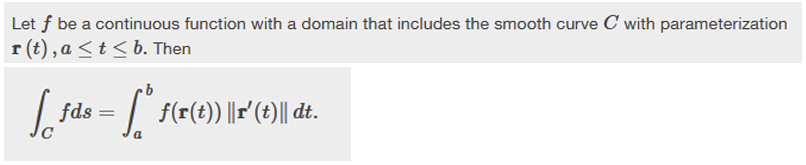
Note that:
The following theorem provides the mechanism to evaluate scalar line integrals:
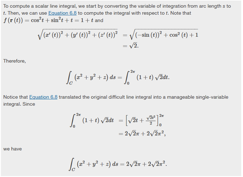
Example:
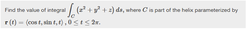
Solution:
Vector Line Integrals
The second type of line integrals are vector line integrals, in which we integrate along a curve through a vector field. For example, let
\[ \mathbf{F}(x,y,z) = P(x,y,z)\mathbf{i} + Q(x,y,z)\mathbf{j} + R(x,y,z)\mathbf{k} \]
be a continuous vector field in \( R^3 \) that represents a force on a particle, and let C be a smooth curve in \( R^3 \) contained in the domain of F.
The following formula provides a means to evaluate vector line integrals.
\[ \int_C F \cdot Tds = \int_a^b F(r(t)) \cdot r’ (t) dt. \]
Note that T represents the unit tangent vector.
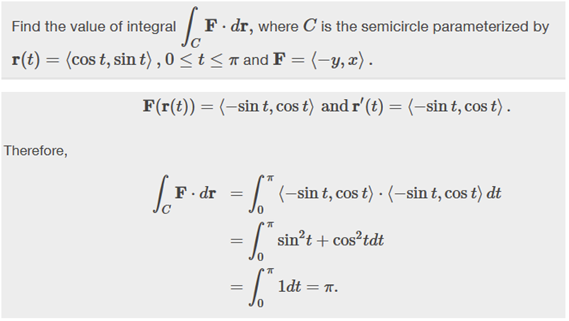
Example:
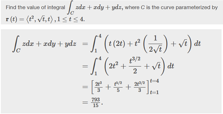
Example:
Applications in Business and Environmental Science
- Business Analytics: Line integrals are applied to compute cumulative cost along a distribution route. Here, the integrand represents cost per unit distance, enabling optimization of delivery paths.
- Environmental Science: When modeling pollutant transport along a river, line integrals integrate concentration along the flow, providing insights into total pollutant mass reaching a downstream location.
