Overview of Limits in Calculus

A limit is one of the most important building blocks of calculus. Essentially, a limit describes what value a function approaches as the input gets closer and closer to a particular point, even if the function never actually reaches that value.
In calculus, limits provide the foundation for both derivatives and integrals. A derivative measures instantaneous change—like finding the slope of a curve at a single point—and this idea is formally defined using limits. Similarly, an integral represents the accumulation of infinitely many small quantities, such as the area under a curve, and limits make this process precise.
In addition, limits help us make sense of situations where direct substitution does not work, such as dividing by zero or dealing with values that approach infinity
Understanding limits allows us to move from algebra’s focus on exact values to calculus’s focus on continuous change and approximation.
The video below provides more details and explanations for using limits and includes several examples to illustrate how to calculate limits as x approaches a certain value, or as x approaches infinity. Both a numerical and graphical approach to limits are discussed.
Introduction to Limits
Calculus is often described as the mathematics of change, and limits provide the essential language and tools to study this change. A limit describes the behavior of a function as its input approaches a certain value, regardless of whether the function is actually defined at that value. This concept allows us to extend mathematics into new territory, such as describing instantaneous rates of change, dealing with infinite processes, and understanding continuity. Without limits, the ideas of derivatives and integrals—the two cornerstones of calculus—cannot be properly defined.
Formal and Intuitive Definitions
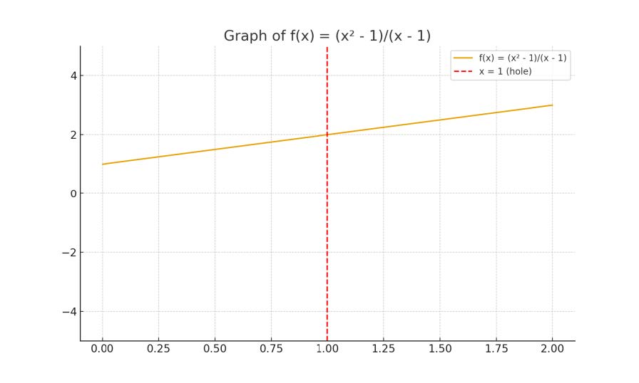
Intuitively, a limit is the value that a function approaches as the input approaches some number. For example, consider f(x) = (x2 – 1)/(x – 1). If you plug in x = 1 directly, you obtain 0/0, which is undefined. However, if you compute values of f(x) for x near 1 (such as 0.9, 0.99, 1.01, 1.1), you will notice that f(x) approaches 2. We therefore say the limit as x approaches 1 is 2, even though the function itself is not defined at x = 1.
Numerical and Graphical Approaches
Numerical methods involve constructing a table of values for x that approach the point of interest. This allows us to see how f(x) behaves. For example:
Consider f(x) = sin(x)/x. The function is not defined at x = 0, but we can compute values for x approaching 0:
x = 0.1 → f(x) ≈ 0.998
x = 0.01 → f(x) ≈ 0.99998
x = -0.1 → f(x) ≈ 0.998
x = -0.01 → f(x) ≈ 0.99998
From both sides, the function approaches 1, so lim (sin(x)/x) as x → 0 is 1.
Graphical methods involve looking at the curve and observing what value the function approaches as x gets close to the point of interest. Graphs are particularly useful for developing an intuitive understanding of limit.
One-Sided vs. Two-Sided Limits
A two-sided limit exists if and only if both one-sided limits exist and are equal. The left-hand limit (as x approaches from values less than c) is written as lim f(x) as x → c⁻. The right-hand limit (as x approaches from values greater than c) is written as lim f(x) as x → c⁺.
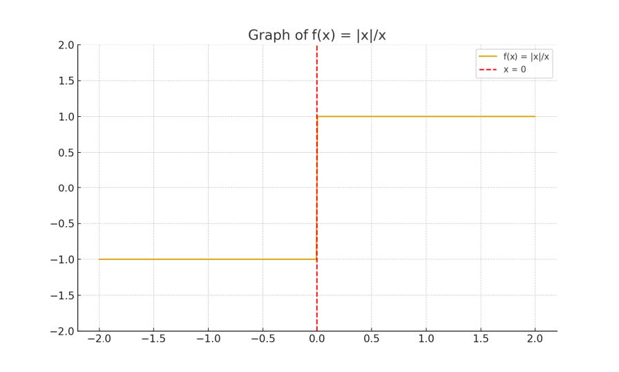
Example: f(x) = |x|/x.
As x → 0⁻ (from the left), f(x) = -1.
As x → 0⁺ (from the right), f(x) = 1.
Because the one-sided limits are not equal, the two-sided limit as x → 0 does not exist.
This illustrates that agreement between both sides is essential for a two-sided limit.
Limits as x → c
When evaluating limits as x approaches a finite number c, the most common approaches include:
- Direct substitution: If f is continuous at c, then lim f(x) = f(c).
- Algebraic simplification: Factor expressions to cancel terms.For example, lim (x2 – 4)/(x – 2) as x → 2 gives 0/0 directly, but factoring the numerator as (x – 2)(x + 2) and canceling the factor (x – 2) on the top and bottom of the fraction results in the limit as x → 2 of (x + 2) which means the limit is 4.
- Rationalization: Multiply numerator and denominator by a conjugate to simplify.
- Piecewise functions: Evaluate each piece and confirm left and right limits agree.
These methods reveal that the actual value of f(c) (or whether f(c) is even defined) has no bearing on the existence of the limit.
Limits as x → ∞ and –∞
Limits at infinity describe how functions behave as x grows arbitrarily large in the positive or negative direction.
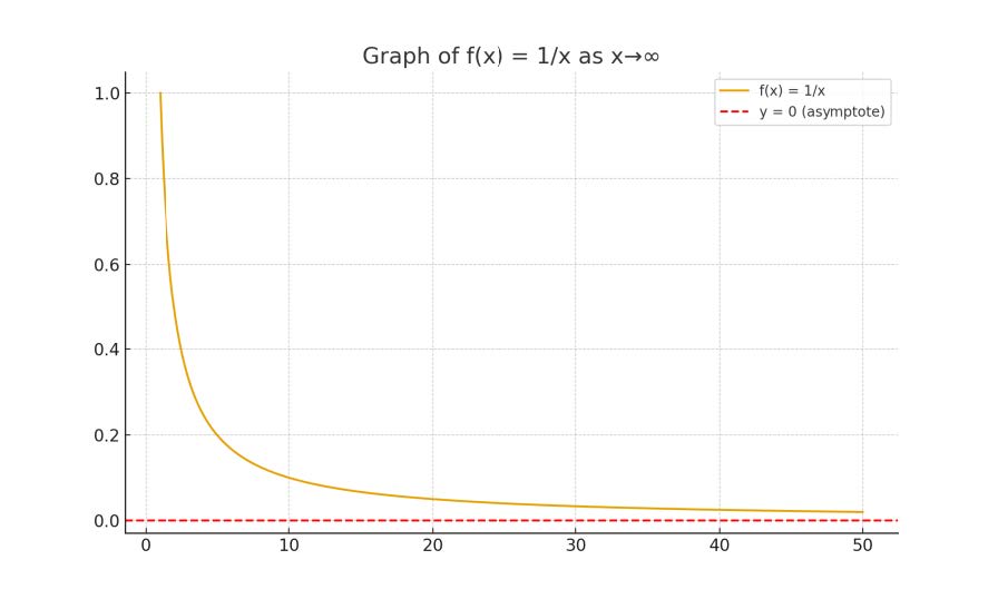
Example 1: lim (1/x) as x → ∞ = 0, since 1/x gets closer and closer to zero.
Example 2: lim (2×2 + 3)/(x2 – 5) as x → ∞. Divide numerator and denominator by x2: (2 + 3/x2)/(1 – 5/x2). As x → ∞, this approaches 2/1 = 2.
Example 3: lim (5×3)/(2×2) as x → ∞. Because the numerator grows faster, the limit is ∞.
Horizontal asymptotes of rational functions can be determined by limits at infinity, while vertical asymptotes occur when limits at finite points diverge.
Key Theorems and Properties of Limits
Several important properties make limits powerful tools:
- Sum Rule: lim (f(x) + g(x)) = lim f(x) + lim g(x).
- Product Rule: lim (f(x)·g(x)) = (lim f(x))·(lim g(x)).
- Quotient Rule: lim (f(x)/g(x)) = (lim f(x))/(lim g(x)), provided lim g(x) ≠ 0.
- Constant Multiple Rule: lim (k·f(x)) = k·lim f(x).
These theorems allow evaluation of more complicated limits.
Examples and Worked Problems
Example 1: lim (x2 – 1)/(x – 1) as x → 1.
Direct substitution → 0/0. Factor: (x – 1)(x + 1)/(x – 1). Cancel (x – 1). Limit = 2.
Example 2: lim (1/x) as x → ∞.
As x grows larger, 1/x → 0. Limit = 0.
Example 3: lim |x|/x as x → 0.
Left-hand limit = -1, right-hand limit = 1, so two-sided limit does not exist.
Example 4: Graphical interpretation.
Suppose f(x) has a hole at x = 2 but approaches value 5 from both sides. Then lim f(x) as x →
2 = 5, regardless of whether f(2) is defined.
Example 5: Infinite limits.
lim (1/(x – 2)) as x → 2⁺ = +∞, lim (1/(x – 2)) as x → 2⁻ = -∞.
Summary and Applications
Limits provide the foundation for continuity, derivatives, and integrals. They allow us to rigorously define instantaneous change and accumulation, two core ideas of calculus. The study of limits reveals that what matters most is the behavior of a function near a point, not necessarily its value at that point. Thus, the existence or nonexistence of f(c) at x = c has no bearing on the existence of lim f(x) as x → c. This distinction is essential in both theory and application, making limits a central concept for all further topics in calculus.
Graphs Illustrating Limits
The following graphs provide visual intuition for different types of limits:
1. A rational function with a removable discontinuity:
2. A rational function with a horizontal asymptote as x → ∞:
3. A piecewise function with different one-sided limits at x = 0:
Numerical Table Example
Consider f(x) = sin(x)/x as x → 0. We can estimate the limit numerically by using a table:
| x | f(x) = sin(x)/x |
| 0.1 | 0.99833 |
| 0.01 | 0.99998 |
| -0.1 | 0.99833 |
| -0.01 | 0.99998 |
