Taylor Polynomials

In this section, we review a special type of series which involve variables. A power series is a series which involves powers of x, such as x2, x3, etc.
A common power series is as follows:
A power series can be thought of as an infinite polynomial.
Power series are used to represent common functions such as sin(x), cos(x) and ex. In fact, these power series are the basis of how a handheld calculator provides a numeric result for these functions on the calculator.
Power series can also be used to generate and define new functions. In this section we define power series and show how to determine when a power series converges and when it diverges. We also show how to represent certain functions using power series. We will introduce the concept of a Taylor polynomials which will allow us to show how polynomial functions can be used as approximations for other elementary functions.
A Taylor series will be a power series which makes use of various derivatives of a given function, such as first, second, third derivatives.
The Taylor series representation is written as:
This power series for f is known as the Taylor series for f at a.
Taylor series allows us to write power series to represent various common function such as sin(x), cos(x) and ex.
The video below explores the setup of these Taylor series representations and provides several worked out examples.
Background
Taylor polynomials are a tool in calculus used to approximate complicated functions with simpler polynomial expressions. A Taylor polynomial will be a power series which makes use of various derivatives of a given function, such as first, second, third derivatives. Taylor polynomials are based on the concept that a smooth function can be closely approximated by a polynomial whose coefficients are determined by the function’s derivatives at a specific point. Taylor polynomials provide a local approximation of a function around a chosen point, usually denoted as ‘a’. When the point chosen is a = 0, the Taylor polynomial is often called a Maclaurin polynomial.
Power Series
In general, a power series is a series which involves powers of x, such as x2, x3, etc.
Power series are used to represent common functions such as sin(x), cos(x) and ex. In fact, these power series are the basis of how a handheld calculator provides a numeric result for these functions on the calculator.
Power series can also be used to generate and define new functions. In this section we define power series and show how to determine when a power series converges and when it diverges. We also show how to represent certain functions using power series. We will introduce the concept of a Taylor polynomials which will allow us to show how polynomial functions can be used as approximations for other elementary functions.
A power series is a series of the form:
\[ \sum_{n=0}^{\infty} c_n x^n = c_0 + c_1x + c_2x^2 + \cdots, \]
Where x is the variable and the “c” values are coefficients.
Here are several examples of power series:
\[ \sum_{n=0}^{\infty} \frac{x^n}{n!} = 1 + x + \frac{x^2}{2!} + \frac{x^3}{3!} + \cdots \]
\[ \sum_{n=0}^{\infty} n!x^n = 1 + x + 2!x^2 + 3!x^3 + \cdots \]
Recall that the series:
\[ \sum_{n=0}^{\infty} x^n = 1 + x + x^2 + \cdots \]
Taylor Series
Taylor polynomials provide approximations of functions that are otherwise difficult to evaluate. They are used in physics, engineering, economics, and numerical methods to simplify computations. For example, when calculators or computers compute trigonometric functions like sin(x) or exponential functions like ex, they often use Taylor polynomial approximations behind the scenes.
The Taylor series representation is written as:
\[ \sum_{n=0}^{\infty} \frac{f^{(n)}(a)}{n!}(x-a)^n = f(a) + f'(a)(x-a) + \frac{f”(a)}{2!}(x-a)^2 + \frac{f”'(a)}{3!}(x-a)^3 + \cdots.\]
This power series for f is known as the Taylor series for f at a.
Taylor series allows us to write power series to represent various common function such as sin(x), cos(x) and ex.
The video below explores the setup of these Taylor series representations and provides several worked out examples.
Rather than construct the infinite series, we can also construct partial sums of Taylor polynomials as follows:
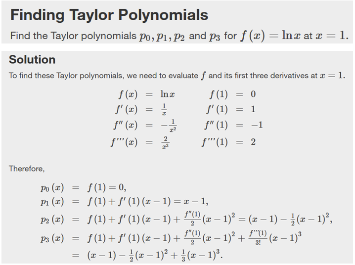
\[ p_0 (x) = f(a), \]
\[ p_1 (x) = f(a) + f'(a)(x-a), \]
\[ p_2 (x) = f(a) + f'(a)(x-a) + \frac{f”(a)}{2!}(x-a)^2, \]
\[ p_3 (x) = f(a) + f'(a)(x-a) + \frac{f”(a)}{2!}(x-a)^2 + \frac{f”'(a)}{3!}(x-a)^3, \]
These partial sums are known as the 0th, 1st, 2nd, and 3rd Taylor polynomials of f at a, respectively
Examples of Taylor Polynomials
Example:
Example:
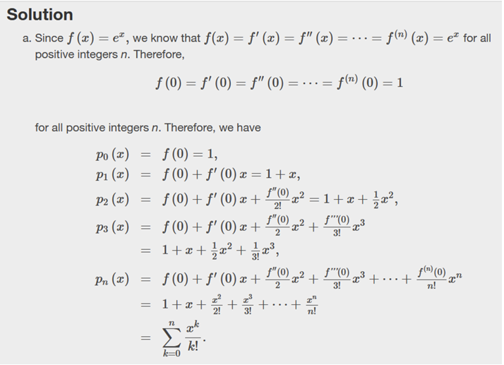
Find the Taylor Polynomial for f(x) = ex about a = 0
Let us approximate the exponential function f(x) = ex using a Taylor polynomial centered at a = 0. Since all derivatives of ex are equal to ex we have fn(0) = 1 for all n.
Thus, the Taylor series for ex is:
\[ P_n(x) = 1 + x + \frac{x^2}{2!} + \frac{x^3}{3!} + \cdots + \frac{x^n}{n!} \]
For example, the 4th degree Taylor polynomial is:
\[ P_4(x) = 1 + x + \frac{x^2}{2} + \frac{x^3}{6} + \frac{x^4}{24} \]
Example:
Find the Taylor Polynomial for f(x) = sin(x) about a = 0
The sine function has derivatives that repeat in a cycle:
f(x) = sin(x), f'(x) = cos(x), f”(x) = -sin(x), f”'(x) = -cos(x), f(4)(x) = sin(x), etc.
Evaluating at x = 0, we get: f(0) = 0, f'(0) = 1, f”(0) = 0, f”'(0) = -1.
Therefore, the Taylor series expansion for sin(x) is:
\[ P_n(x) = x – \frac{x^3}{3!} + \frac{x^5}{5!} – \frac{x^7}{7!} + \cdots \]
For example, the 5th degree polynomial approximation is:
\[ P_5(x) = x – \frac{x^3}{6} + \frac{x^5}{120} \]
Example:
Find the Taylor Polynomial of f(x) = ln(1+x) about a = 0
Consider f(x) = ln(1+x). Its derivatives are:
f'(x) = 1/(1+x), f”(x) = -1/(1+x)2, f”'(x) = 2/(1+x)3, f(4)(x) = -6/(1+x)4, etc.
Evaluating at x = 0, we get: f(0) = 0, f'(0) = 1, f”(0) = -1, f”'(0) = 2, f(4)(0) = -6.
Therefore, the Taylor series for ln(1+x) is:
\[ P_n(x) = x – \frac{x^2}{2} + \frac{x^3}{3} – \frac{x^4}{4} + \cdots + \frac{(-1)^{n+1}x^n}{n} \]
For example, the 4th degree polynomial approximation is:
\[ P_4(x) = x – \frac{x^2}{2} + \frac{x^3}{3} – \frac{x^4}{4} \]
