Three Dimensional Vectors

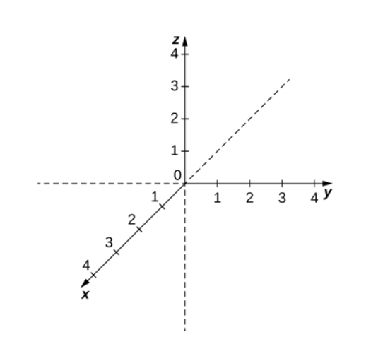
Recall that the two-dimensional rectangular coordinate system contains two perpendicular axes: the horizontal x-axis and the vertical y-axis. We can add a third dimension, the z-axis, which is perpendicular to both the x-axis and the y-axis. We call this system the three-dimensional rectangular coordinate system, as shown below:

Three-dimensional vectors are a fundamental concept in multivariable calculus, providing a method to represent quantities that have both magnitude and direction in space. Unlike two-dimensional vectors that lie in a plane, three-dimensional vectors extend into a third axis, allowing us to model real-world phenomena such as velocity, force, and acceleration in physical space (three-dimensional space). In calculus, vectors are used not only to describe spatial relationships but also to perform operations such as addition, subtraction, and scaling, which form the basis for more advanced calculus applications.

Three-dimensional vectors are also central to understanding vector-valued functions, gradients, directional derivatives, and surface normals. These ideas allow us to analyze how quantities change in multiple directions simultaneously, which is crucial for fields like physics, engineering, and environmental science.

The video below explores the setup of these Maclaurin series representations and provides several worked out examples.

Basics of Three-Dimensional Vectors

A three-dimensional vector is represented by three components, typically denoted as v = ⟨v₁, v₂, v₃⟩, where each component corresponds to the projection of the vector along the x-, y-, and z-axes. Vectors may represent physical quantities such as displacement, velocity, or force. Geometrically, a vector in 3D space can be visualized as an arrow starting from the origin (0, 0, 0) and ending at the point (v₁, v₂, v₃).

The magnitude or length of a vector v = ⟨v₁, v₂, v₃⟩ is given by:

\[ ||v|| = \sqrt{x_1^2 + y_1^2 + z_1^2} \]

Properties of Vectors and Vector Operations

Three-dimensional vectors can be added, subtracted, and multiplied in various ways. The following table summarizes various properties for vectors and vector operations:

Vector Addition and Subtraction

If u = ⟨u₁, u₂, u₃⟩ and v = ⟨v₁, v₂, v₃⟩, then:
u + v = ⟨u₁ + v₁, u₂ + v₂, u₃ + v₃⟩
u − v = ⟨u₁ − v₁, u₂ − v₂, u₃ − v₃⟩

Example: Vector Addition

Let u = ⟨3, −2, 4⟩ and v = ⟨1, 5, −3⟩.

Then:
u + v = ⟨3 + 1, −2 + 5, 4 − 3⟩ = ⟨4, 3, 1⟩.

Scalar Multiplication

If c is a scalar and v = ⟨v₁, v₂, v₃⟩, then multiplying the vector by the scalar gives:
c * v = ⟨c·v₁, c·v₂, c·v₃⟩.

Example: Scalar Multiplication

Let v = ⟨2, −3, 5⟩ and c = 2. Then:
2v = ⟨2·2, 2·(−3), 2·5⟩ = ⟨4, −6, 10⟩.

Unit Vectors:

A unit vector represents a vector of magnitude 1 with the same direction as the original vector.

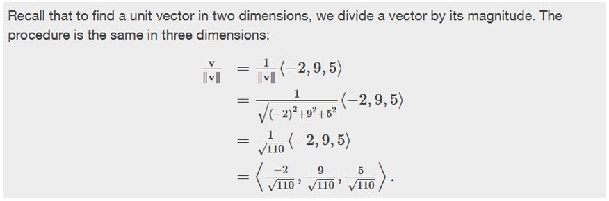
Example: Unit Vector

Let v = ⟨−2,9,5⟩. Find the unit vector in the direction of v.

The unit vector in the direction of the x-axis is labeled as i
The unit vector in the direction of the y-axis is labeled as j
The unit vector in the direction of the z-axis is labeled as k

We can also write these unit vectors as i = ⟨1,0,0⟩, j = ⟨0,1,0⟩, and k = ⟨0,0,1⟩—and we use them in the same way we use the standard unit vectors in two dimensions. Thus, we can represent a vector in three dimensions as:

\[ v = \langle x,y,z \rangle = x\textbf{i} + y\textbf{j} + z\textbf{k}. \]

Writing a Vector extending between two points in 3-dimensional space

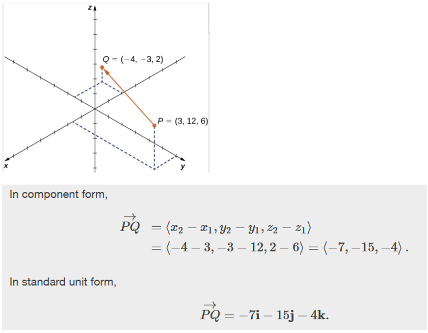
To write the vector extending from points P to Q in three-dimensional space, subtract the corresponding x, y and z components, as shown in the following example:
Let \( \overrightarrow{PQ}\) be the vector with initial point P = (3, 12, 6) and terminal point Q = (−4, −3, 2) as shown in the figure below. Express this vector in both component form and using standard unit vectors i, j, k.

Applications of 3D Vectors in Calculus and Real Life

Three-dimensional vectors have wide-ranging applications. In business, they are used to analyze multidimensional data and model optimization problems. In environmental science, vectors describe wind velocity, pollutant dispersion, and water flow. In physics and engineering, they are typically used for representing forces, motion, and fields.

Example: Business Application – Production Optimization

A company produces three products using three resources: labor, capital, and raw materials. Suppose the resource usage for one unit of each product is represented by vectors:
Product A: ⟨2, 3, 4⟩, Product B: ⟨1, 2, 2⟩, Product C: ⟨3, 1, 5⟩.

If the available resources are represented by the vector ⟨100, 120, 150⟩, the feasibility of a production plan can be tested using vector combinations and scalar multiples to determine if resource limits are exceeded.

Example Environmental Science Application – Wind Flow Analysis

In environmental studies, a wind velocity vector v = ⟨vx, vy, vz⟩ represents the movement of air. Suppose a pollution particle experiences two forces: wind w = ⟨4, −2, 1⟩ and gravity g = ⟨0, 0, −9.8⟩. The net force vector is:

F = w + g = ⟨4, −2, 1 − 9.8⟩ = ⟨4, −2, −8.8⟩.

The resulting vector indicates both the direction and strength of the combined forces acting on the particle.